Differential equations
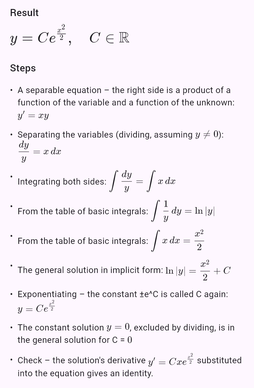
The app solves first-order ordinary differential equations: separable, linear, exact, homogeneous (y′ = f(y/x)), Bernoulli equations and equations y′ = f(ax + by + c). It recognizes the type itself and shows the steps as taught at school – separating the variables, variation of the constant or an integrating factor, a substitution, the potential of an exact equation. The integrals in the steps have steps of their own.
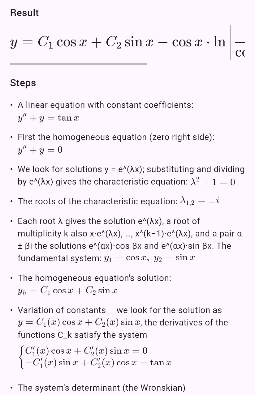
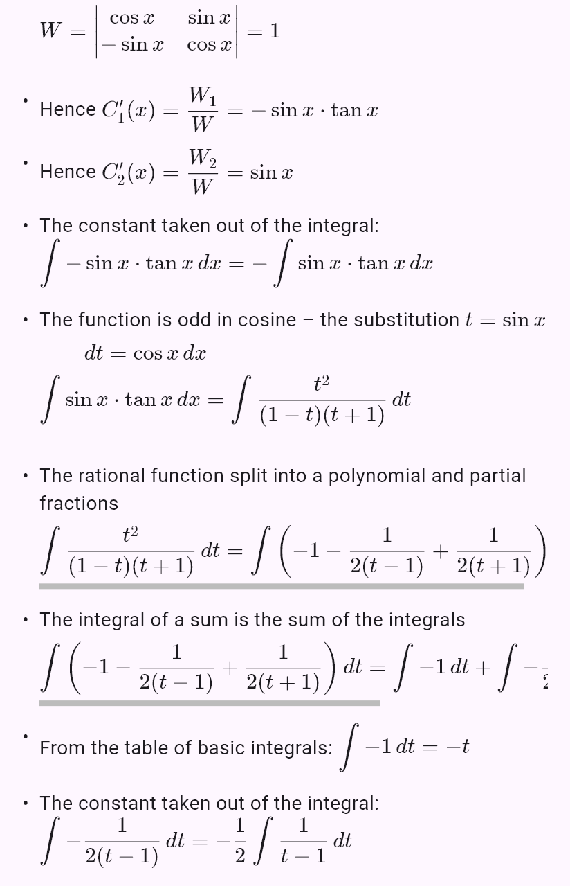
Higher orders: linear equations with constant coefficients of any order by the characteristic equation (multiple and complex roots too), a particular solution by the special right side (resonance and a sum of right sides too) or by variation of constants, an initial value problem at zero by the Laplace transform too (the "Method" chip). Further Euler's equation by x = eᵗ, y⁽ⁿ⁾ = f(x) by repeated integration and the reduction of order – when y is missing (p = y′) or x is (y′ = p(y)).
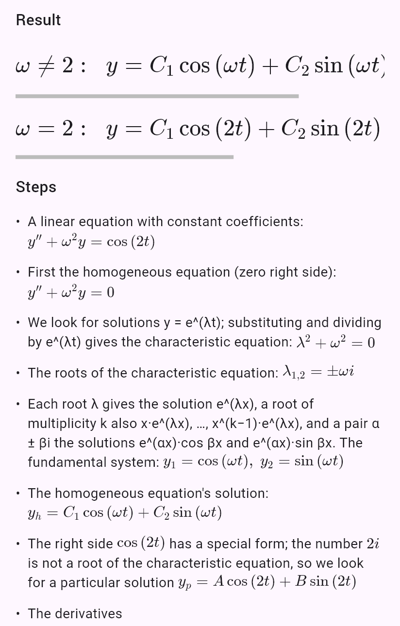
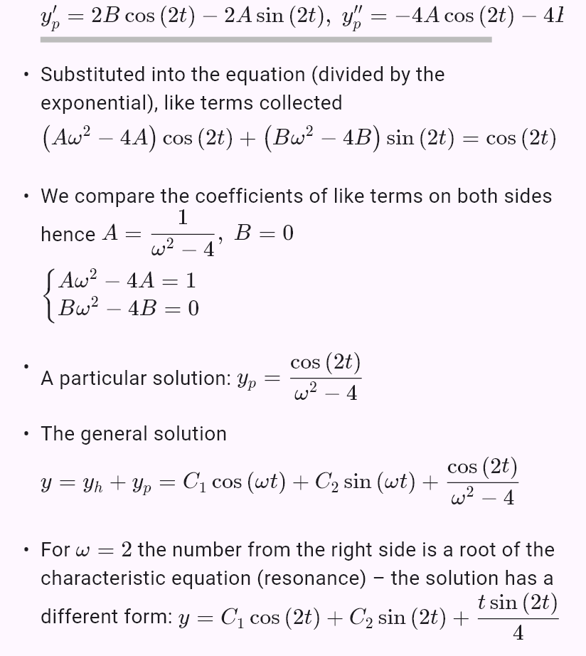
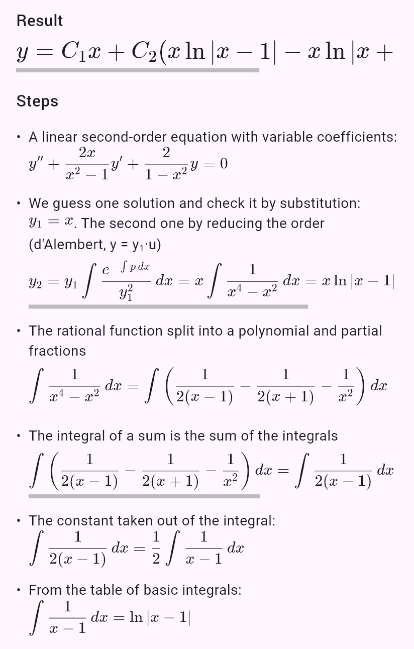
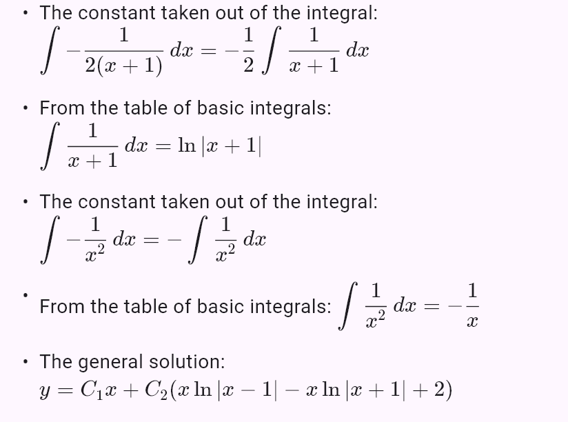
The equation y′ = y·(a(x)·ln y + b(x)) becomes linear by the substitution z = ln y. A linear second-order equation with variable coefficients is solved when one solution can be guessed (xᵏ, eᶜˣ, …): the second one by reducing the order (d'Alembert), the right side by variation of constants. The order is reduced by more than one too (p = y⁽ᵐ⁾ with a second-order equation for p). With parameters the cases are told apart – a damped oscillator by the sign of δ² − ω² (overdamped, critical, underdamped), a resonance (y″ + ω²y = cos 2t for ω = 2) and the sign of a constant the integral depends on (y″ = 2yy′). The Laplace transform also solves an initial value problem at a point other than 0 (by the shift τ = t − t₀) and with parameters.
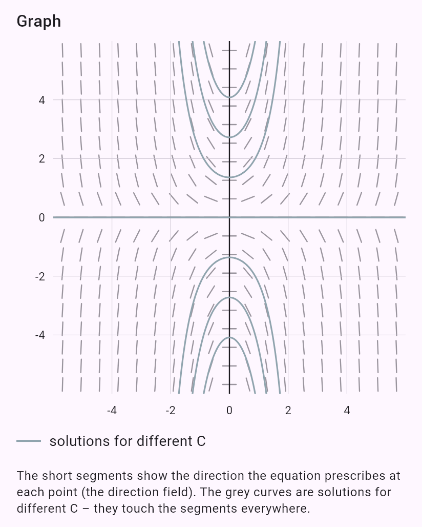
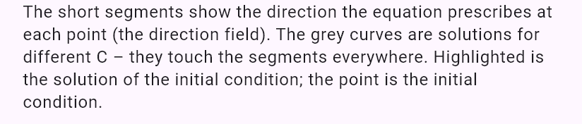
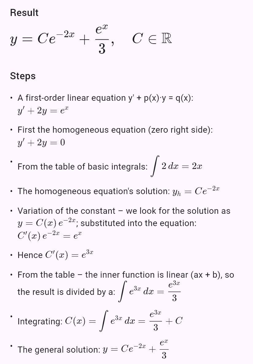
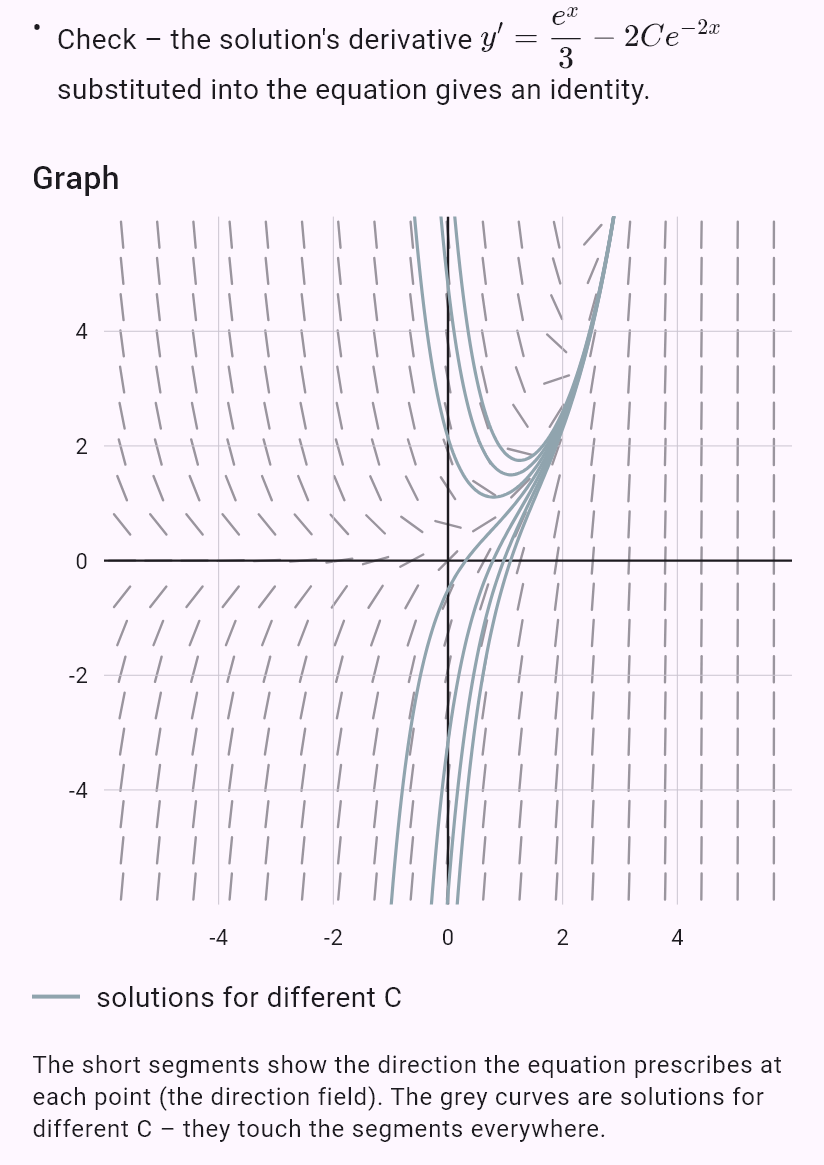
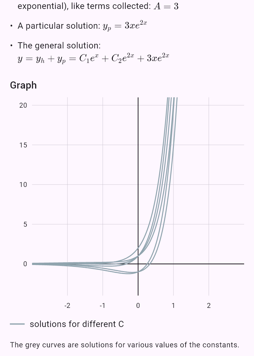
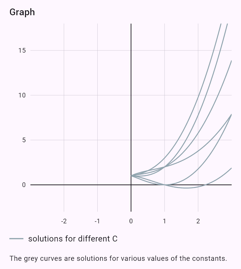
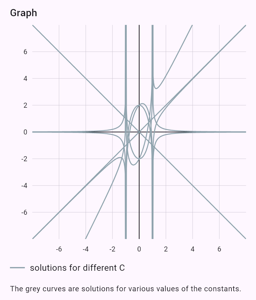
The result is the general solution with a constant C, for higher orders with constants C₁, C₂, … (explicitly, or implicitly where it can't be explicit); with conditions, the solution that satisfies them – initial and boundary ones, including "no solution" and "infinitely many solutions". Constant solutions lost by dividing are found too. Every solution is checked by substituting it into the equation. For the first order the graph shows the direction field and solutions for different C, for higher orders solutions for different constants; for an autonomous second-order equation (no x) a switch shows the phase plane (y, y′) too.
How to enter it
y' = x*y | The derivative with a prime. |
dy/dx = x y^2 | Leibniz's notation – it names the variable too (dm/dt, dT/dt). |
\frac{dy}{dx} = \frac{y}{x} + x | Notation from a photo. |
(2xy + 6x)dx + (x^2 + 4y^3)dy = 0 | The form M dx + N dy = 0 (an exact equation). |
y' = y^2 + 1, y(0) = 1 | An initial condition after a comma or on the next line. |
dm/dt = m + 2, m(0) = 0 | The function and the variable can be any letters. |
y'' - 3y' + 2y = 3e^(2x) | A higher-order equation – the derivatives with more primes. |
y^{(4)} + 2y'' + y = 0 | Higher derivatives as y^{(4)} (from a photo too). |
y'' + y = 0, y(0) = 1, y'(0) = 2 | Initial conditions y(0), y′(0) – or boundary ones at different points. |
\ddot{x} + \omega^2 x = 0 | Newton's dots (derivatives by time t) and Greek parameters. |
Examples
y' = x*y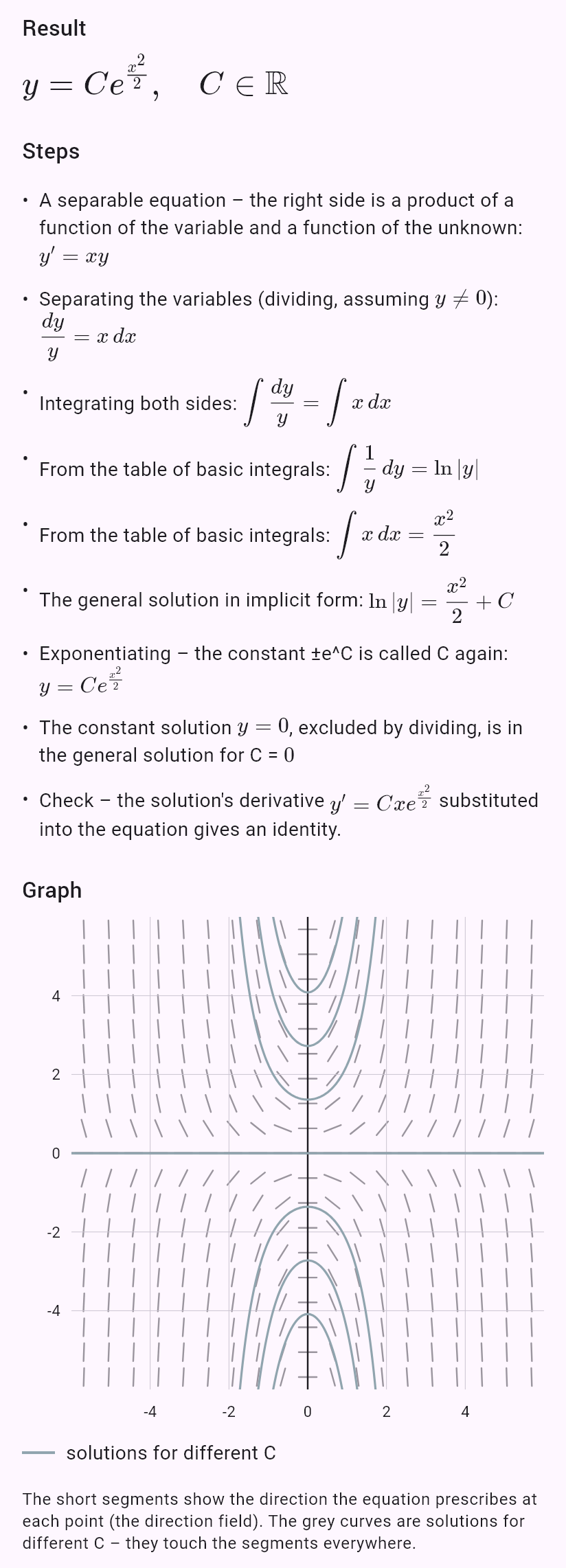
y' = y^2 + 1, y(0) = 1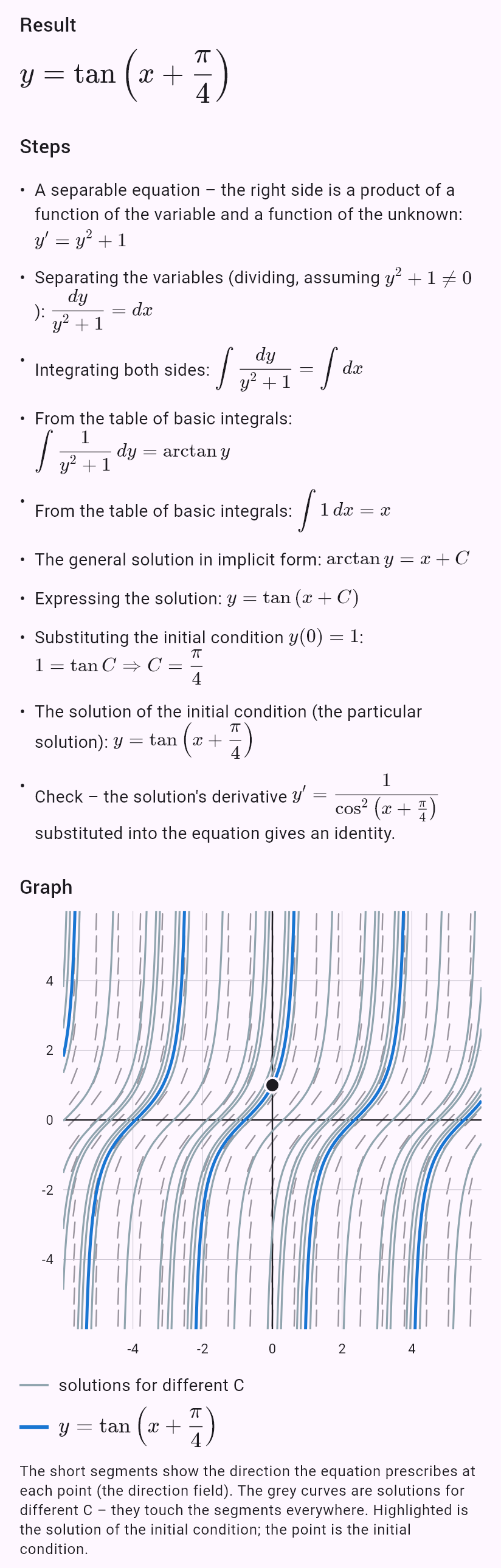
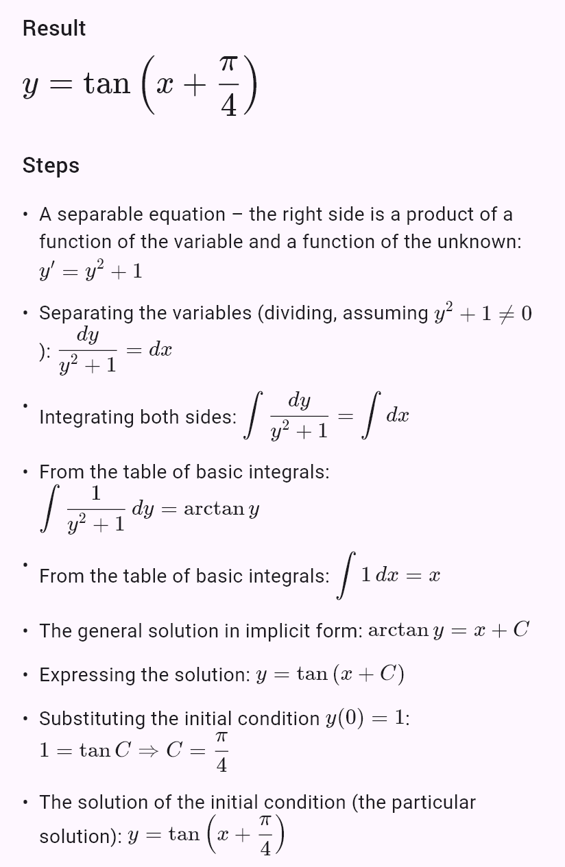
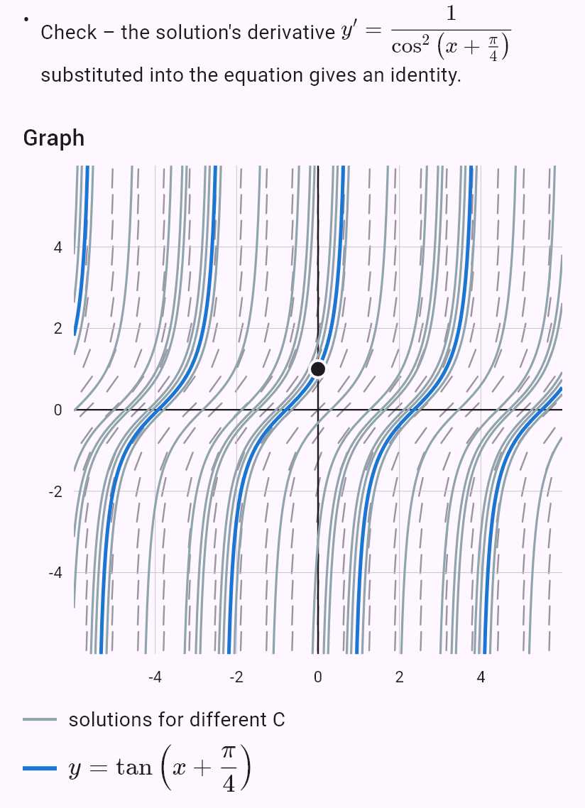
y' + 2y = e^x Variation of the constant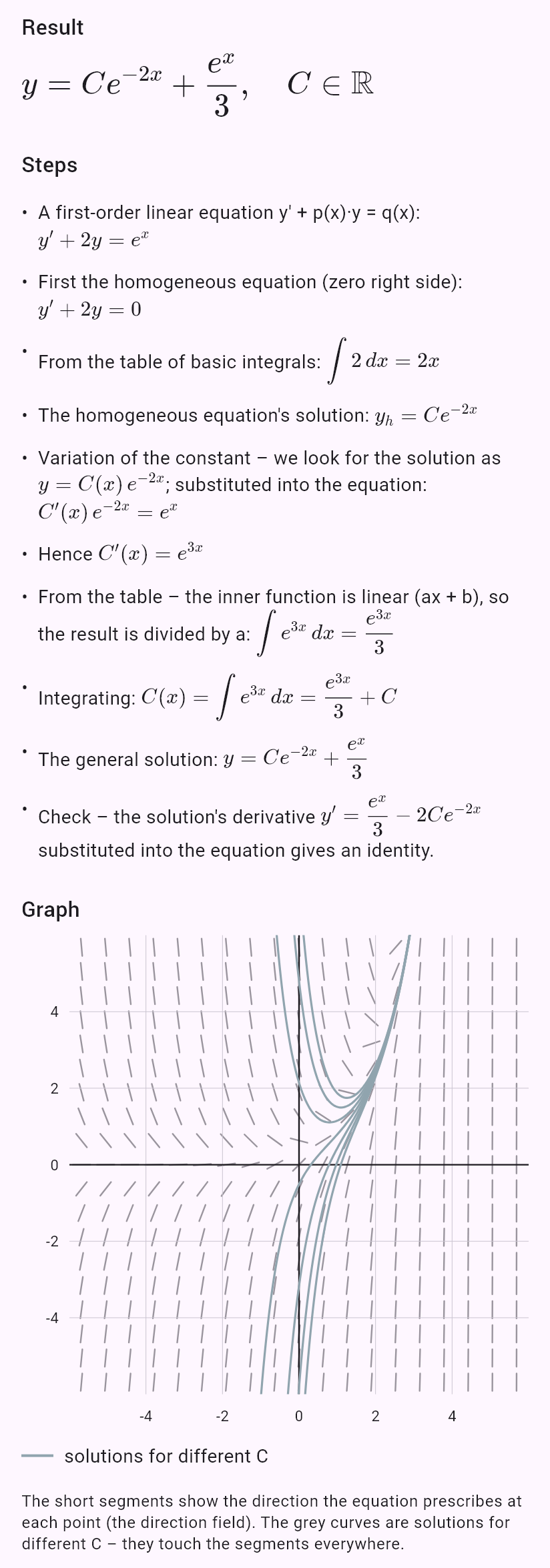
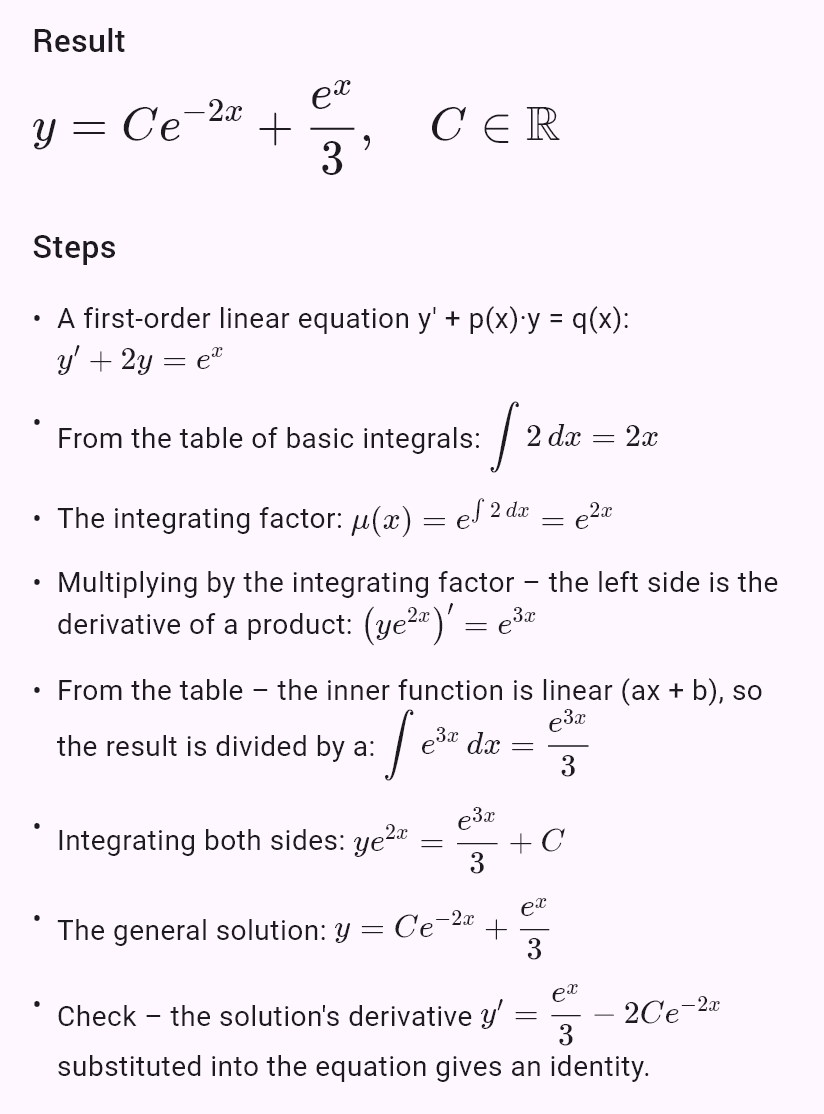
y' + 2y = e^x Integrating factor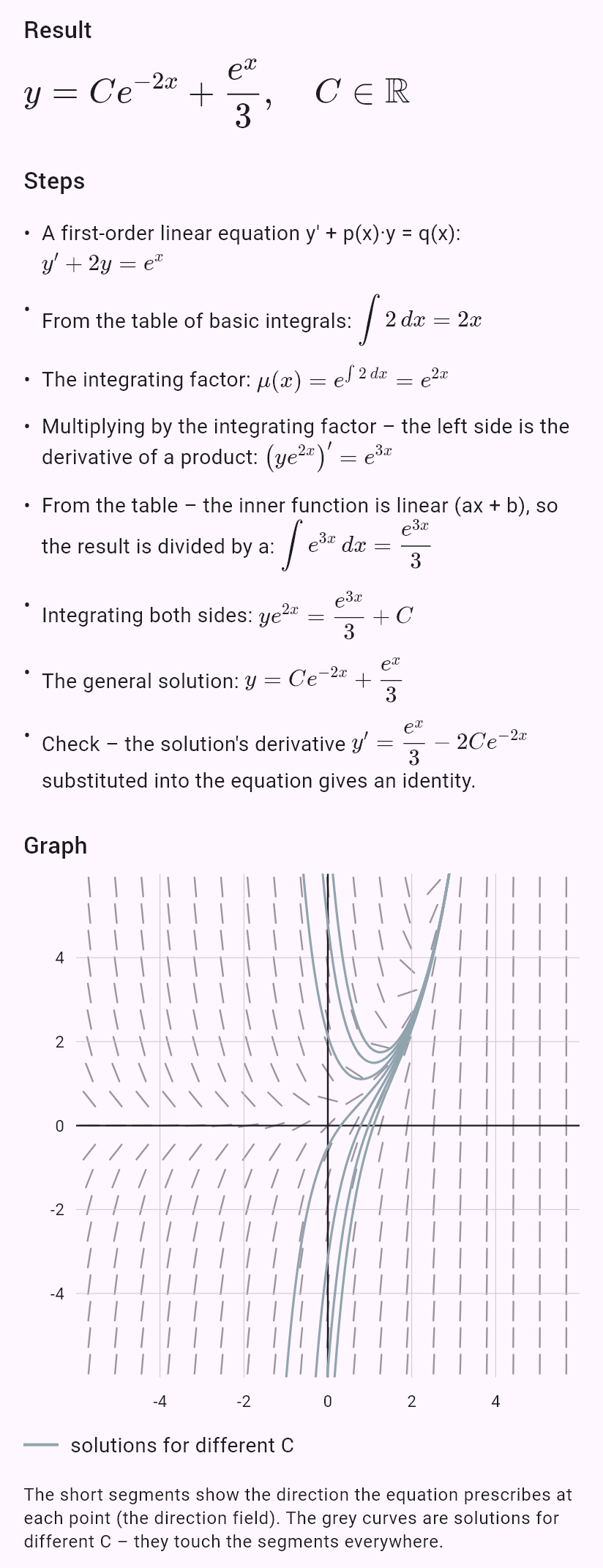
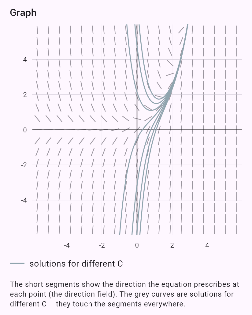
y' = (x - y)/(x + y)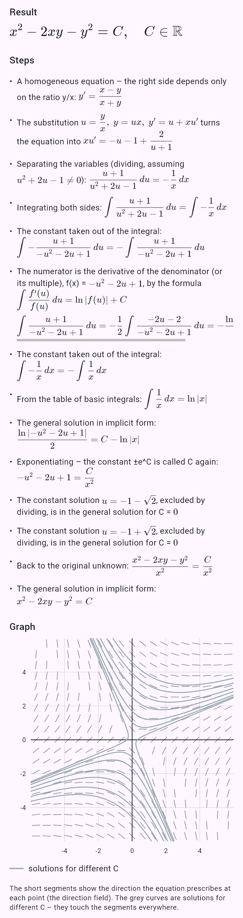
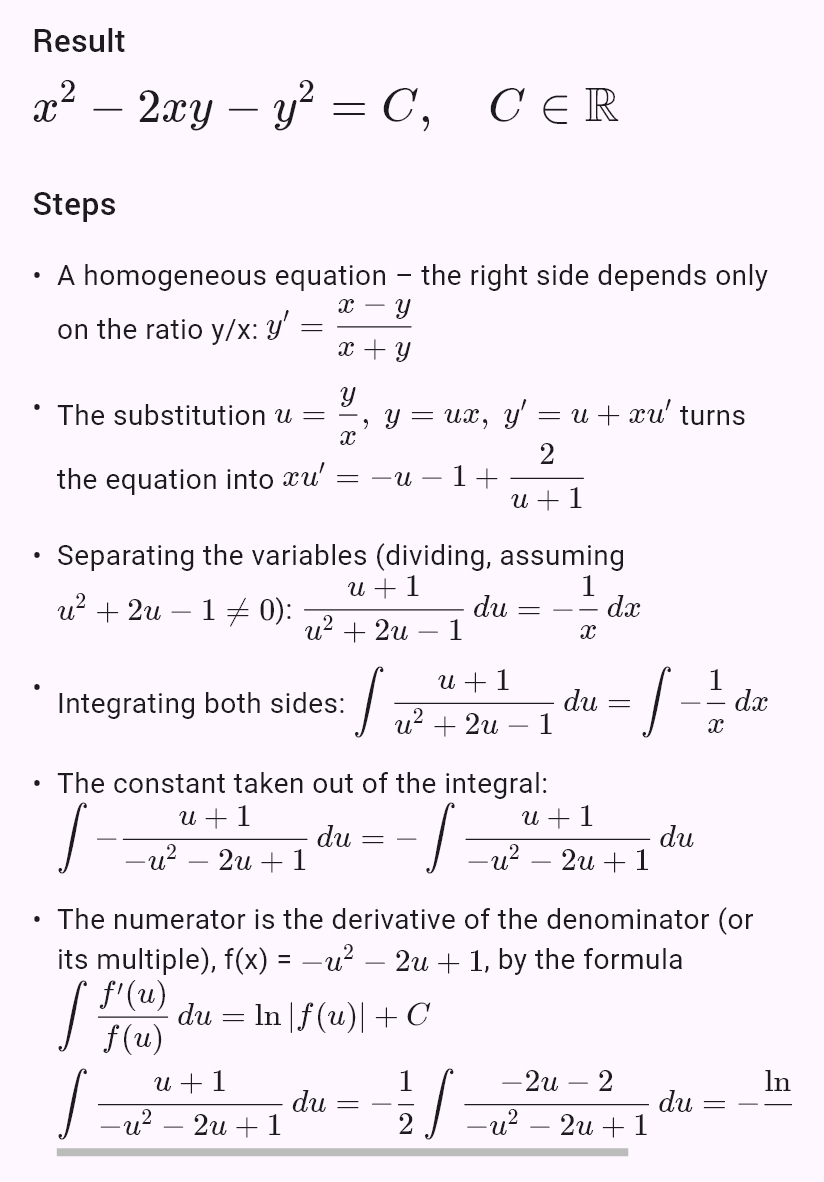
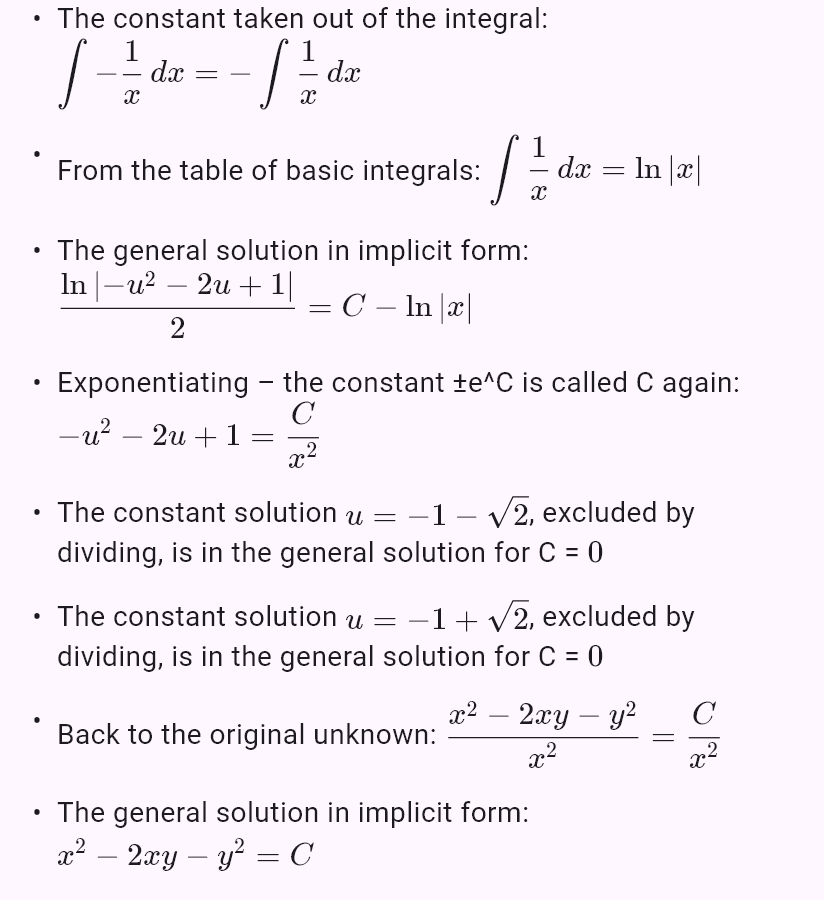
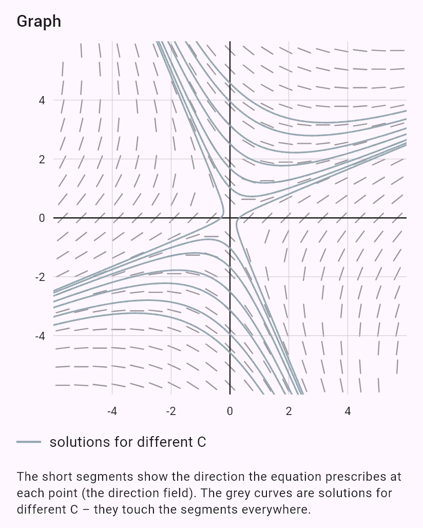
xy' - y = -xy^2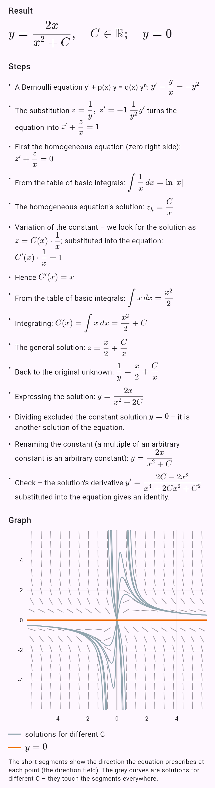
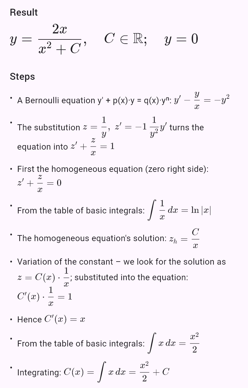
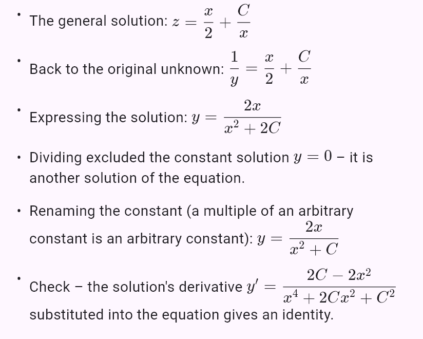
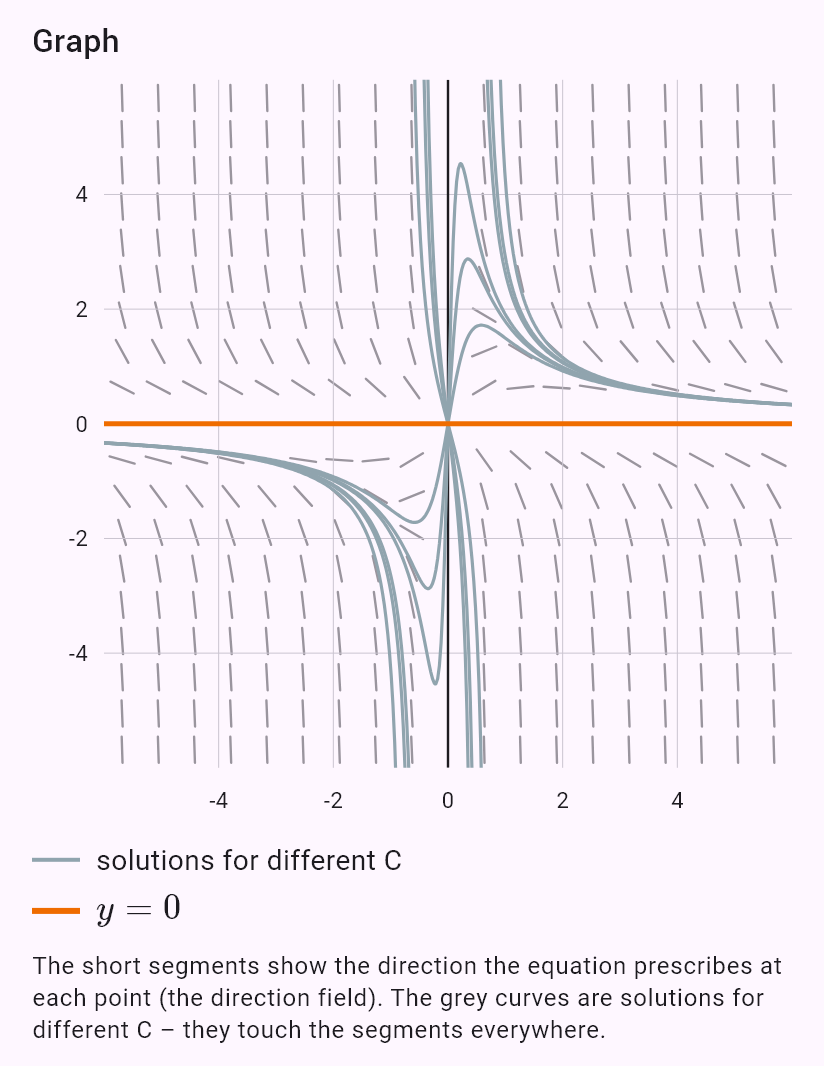
(2xy + 6x)dx + (x^2 + 4y^3)dy = 0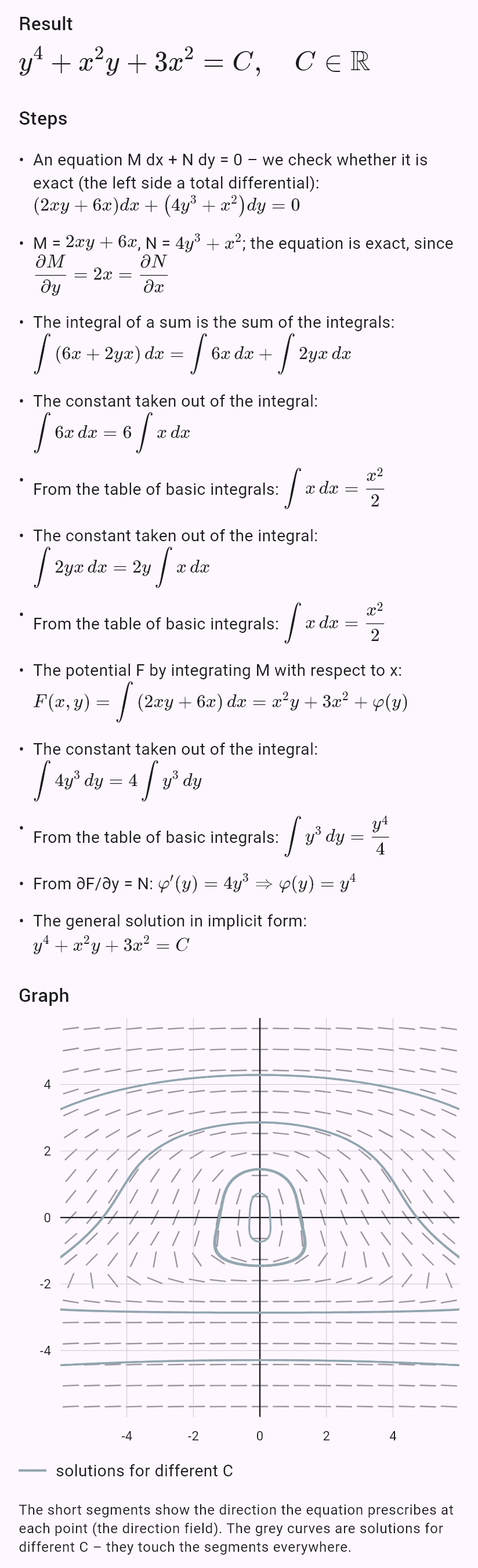
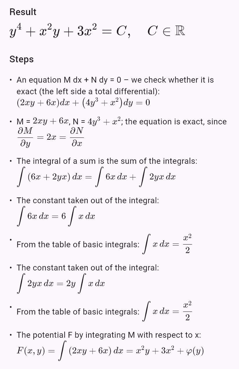
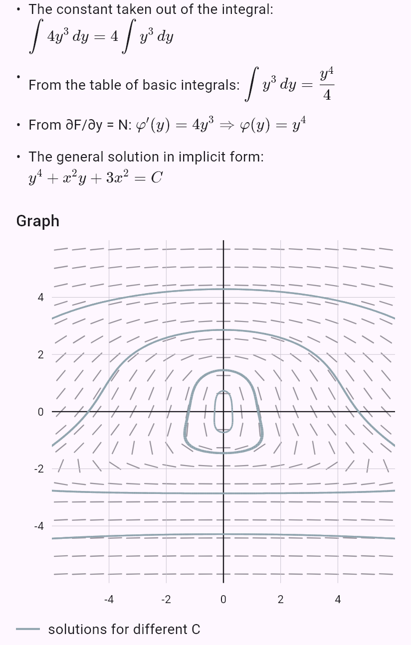

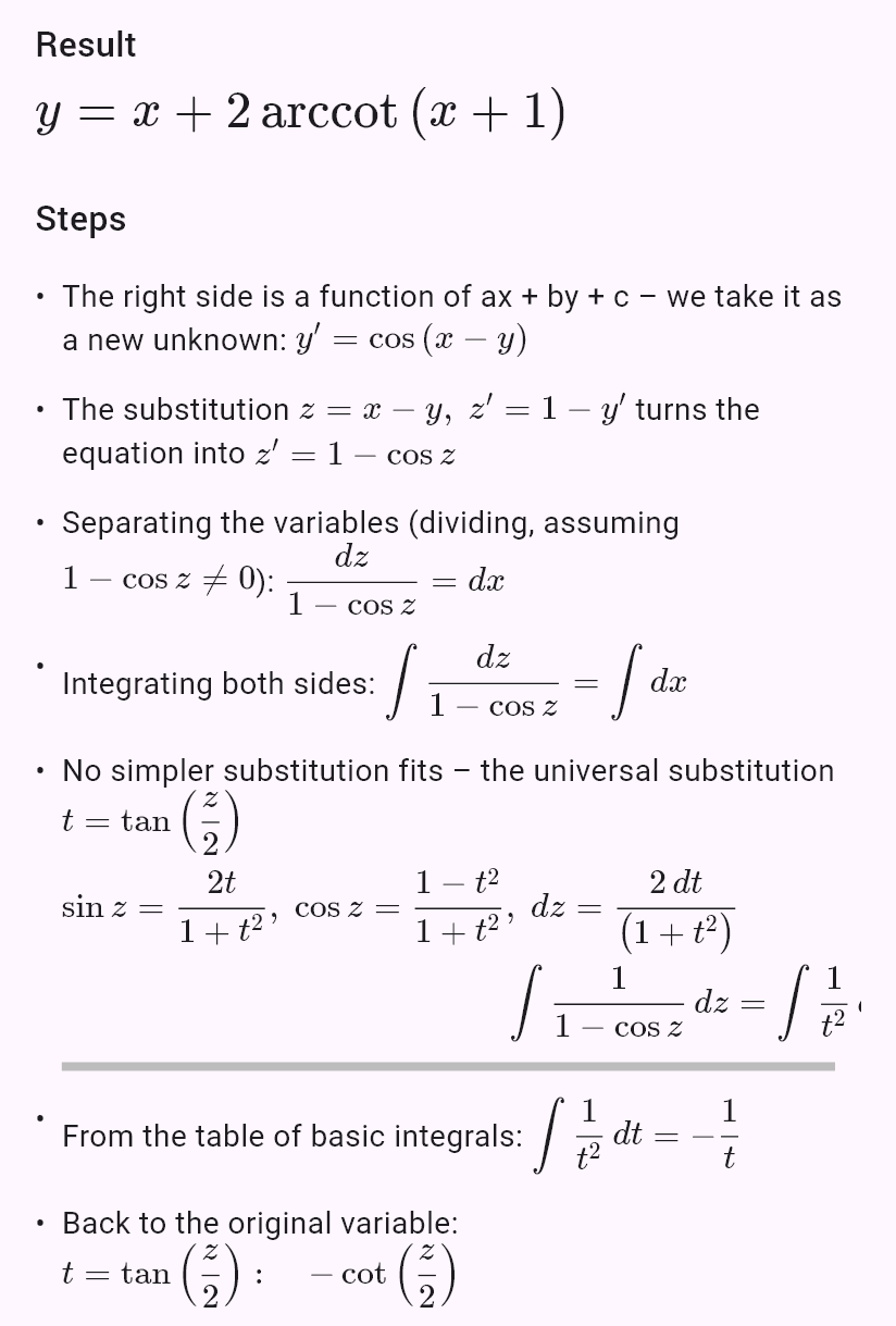
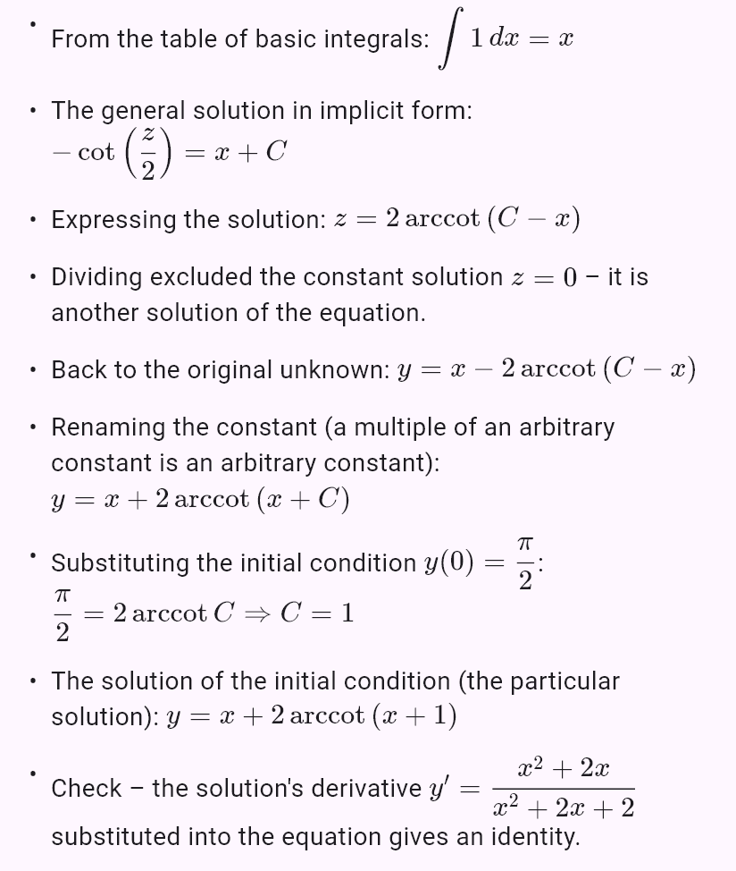
y' = cos(x - y), y(0) = pi/2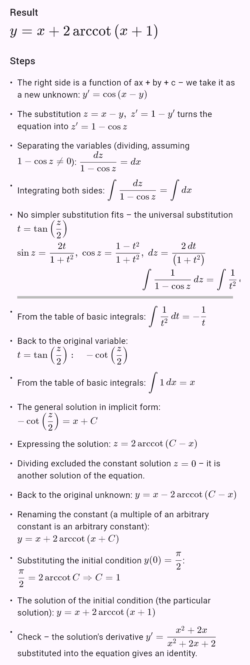
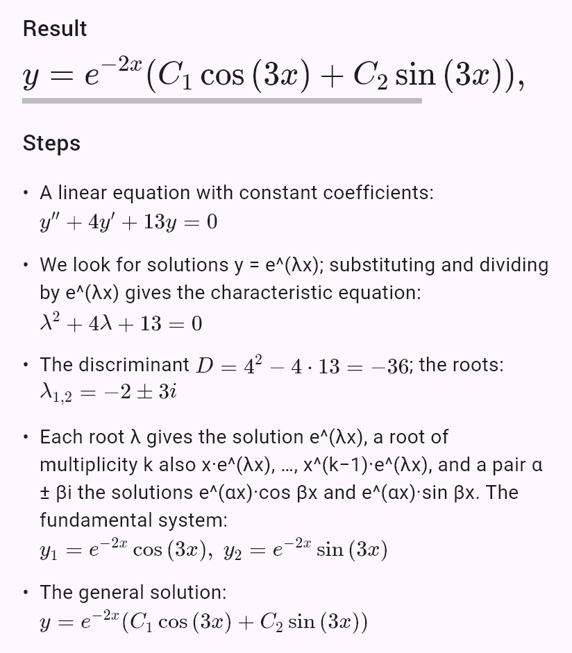
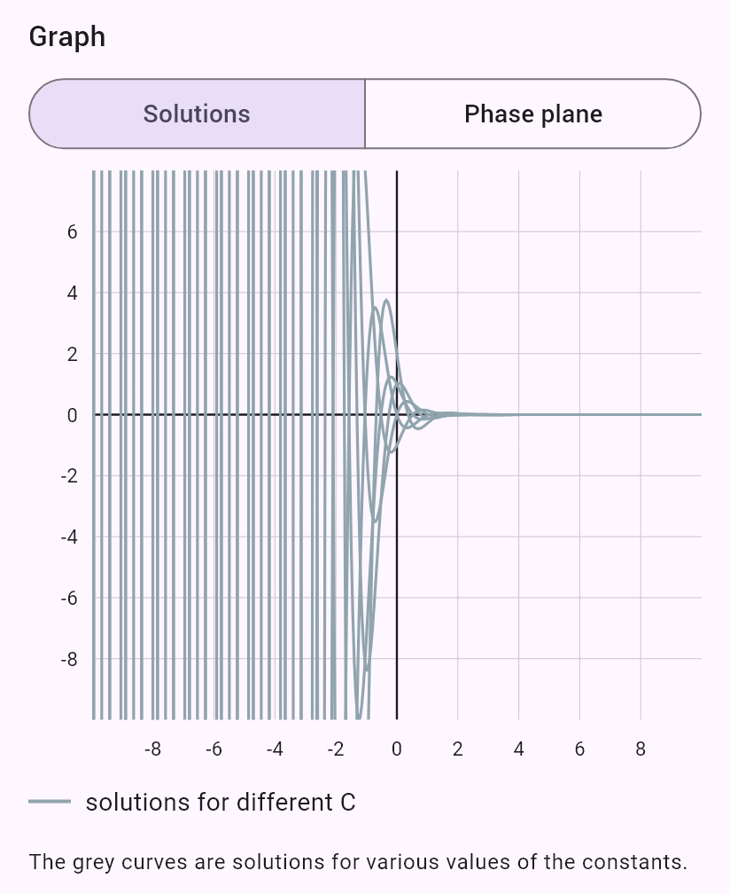
y'' + 4y' + 13y = 0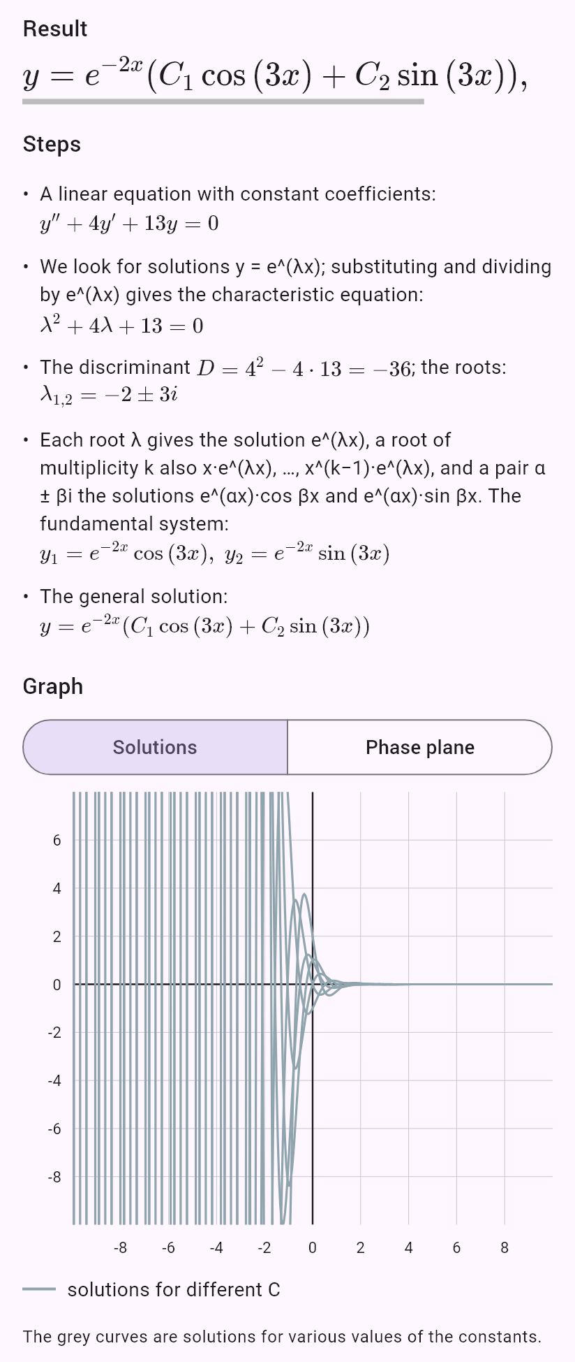
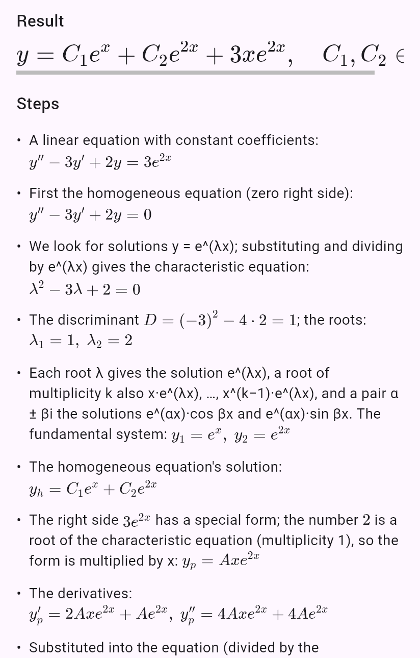
y'' - 3y' + 2y = 3e^(2x) Special right side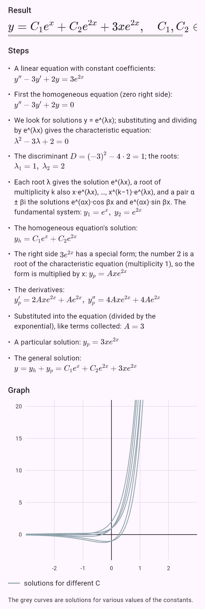
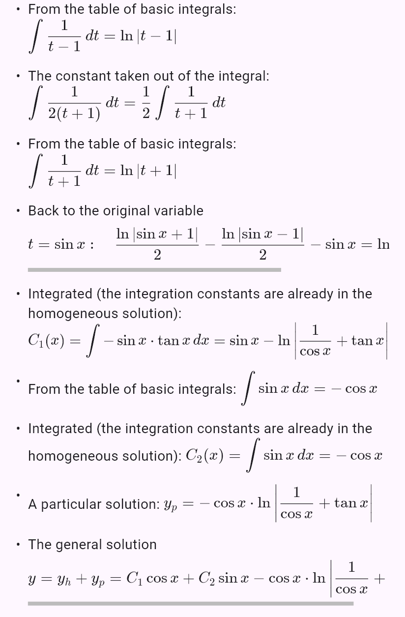
y'' + y = tan x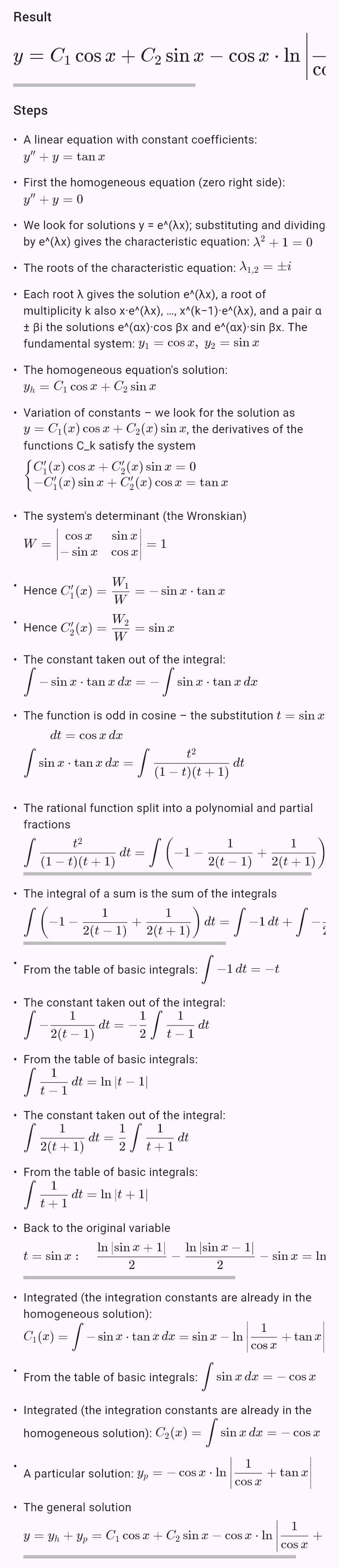
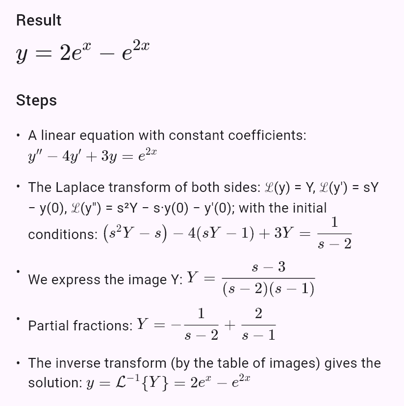
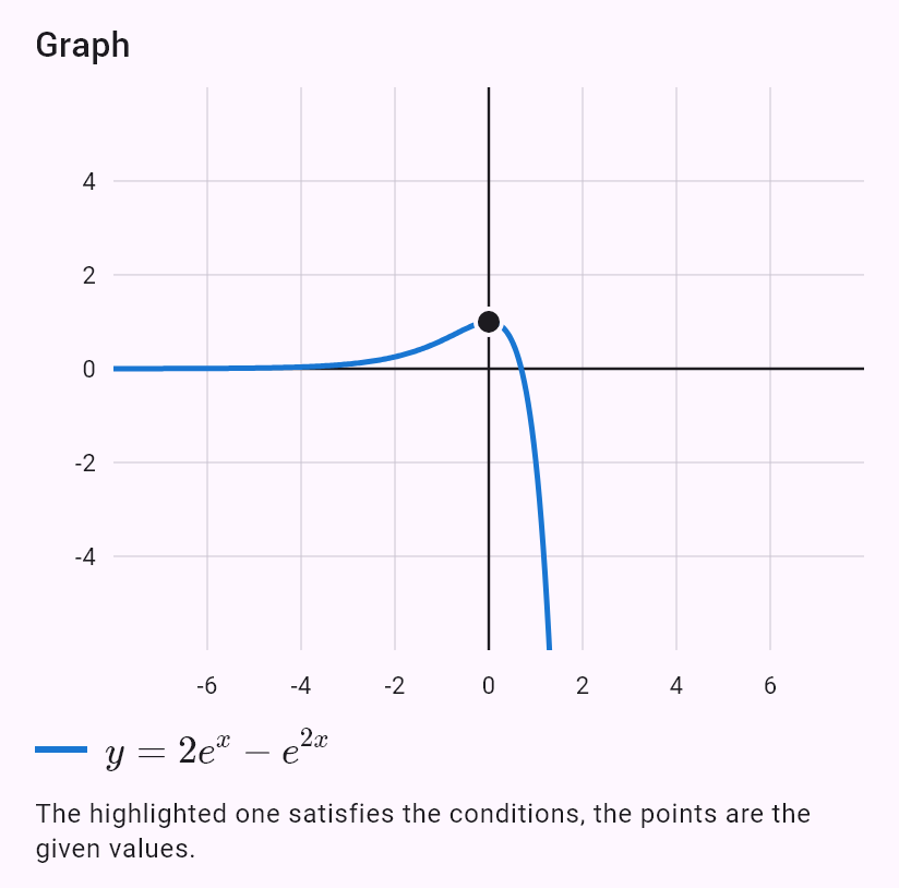
y'' - 4y' + 3y = e^(2x), y(0) = 1, y'(0) = 0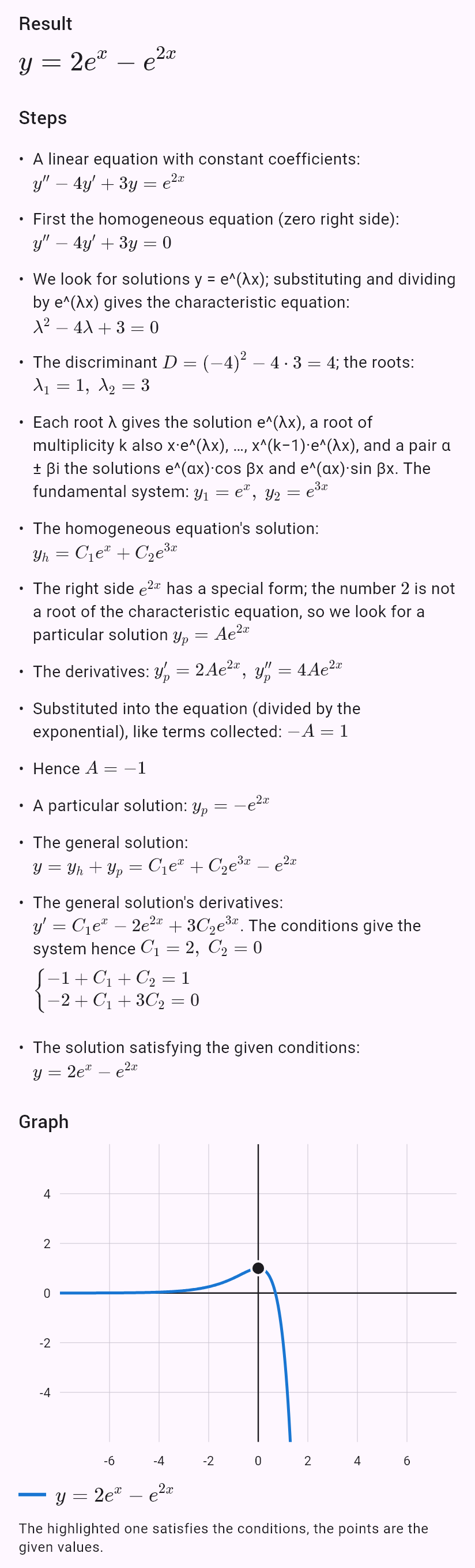
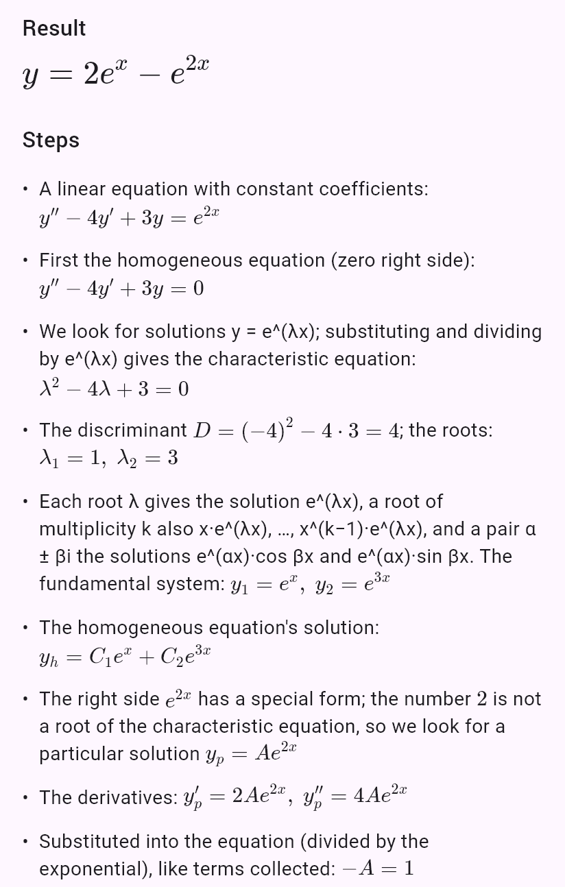
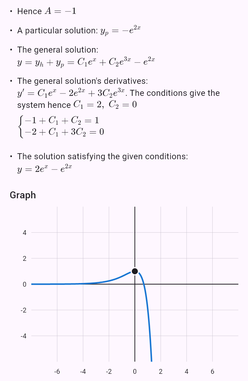

y'' - 4y' + 3y = e^(2x), y(0) = 1, y'(0) = 0 Laplace transform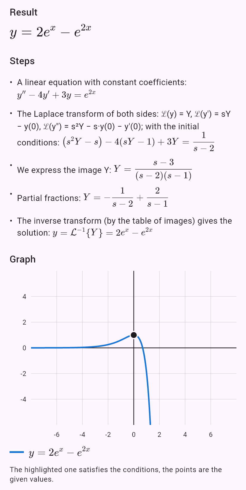
y'' + y = 0, y(0) = 0, y(pi) = 0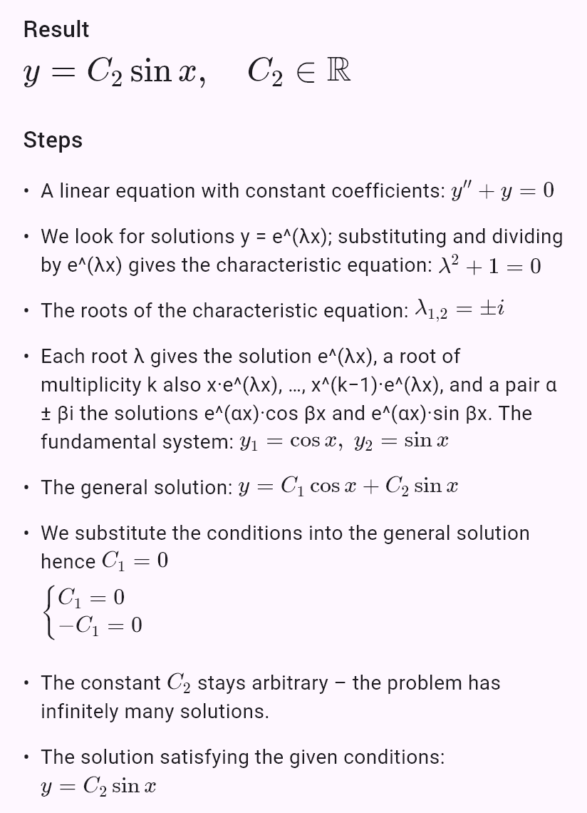
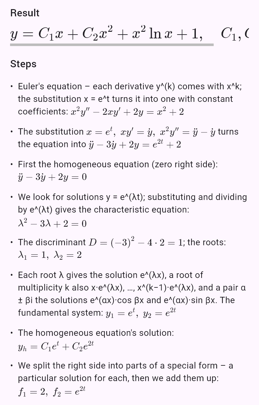
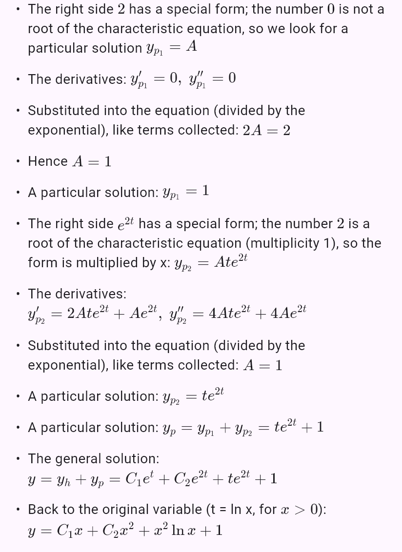
x^2y'' - 2xy' + 2y = x^2 + 2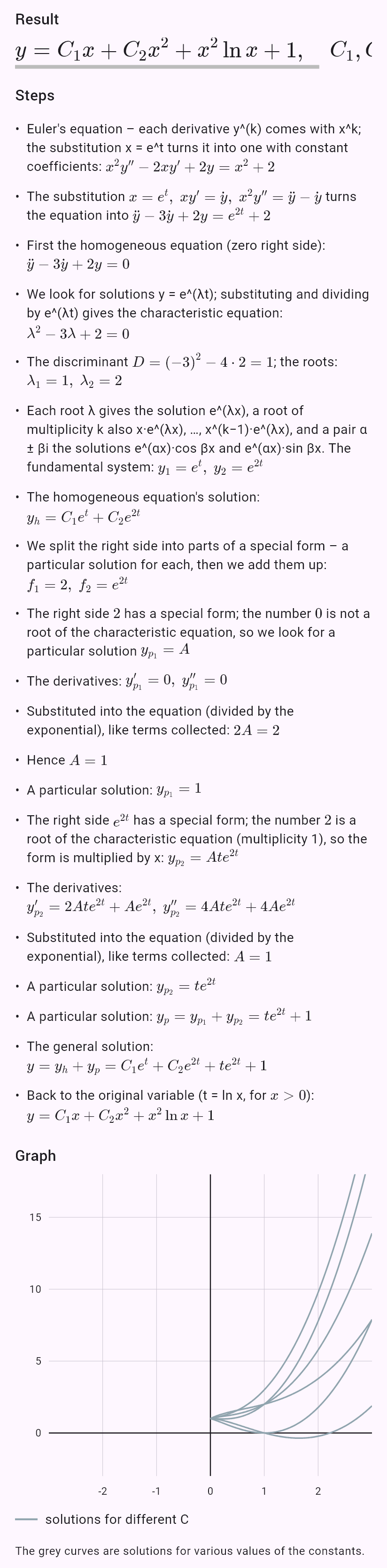
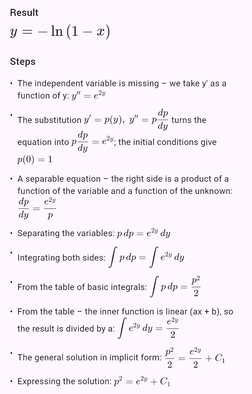
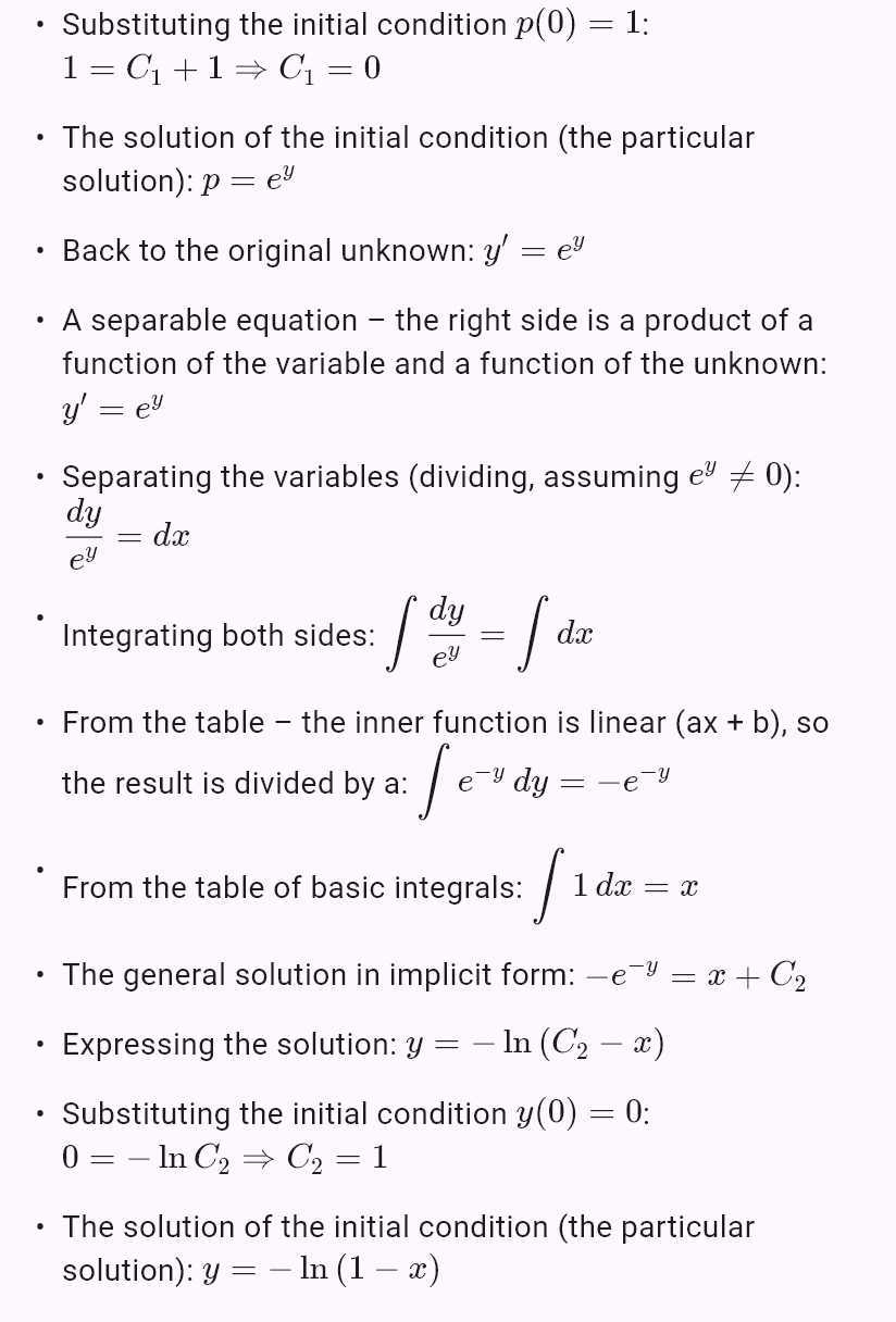
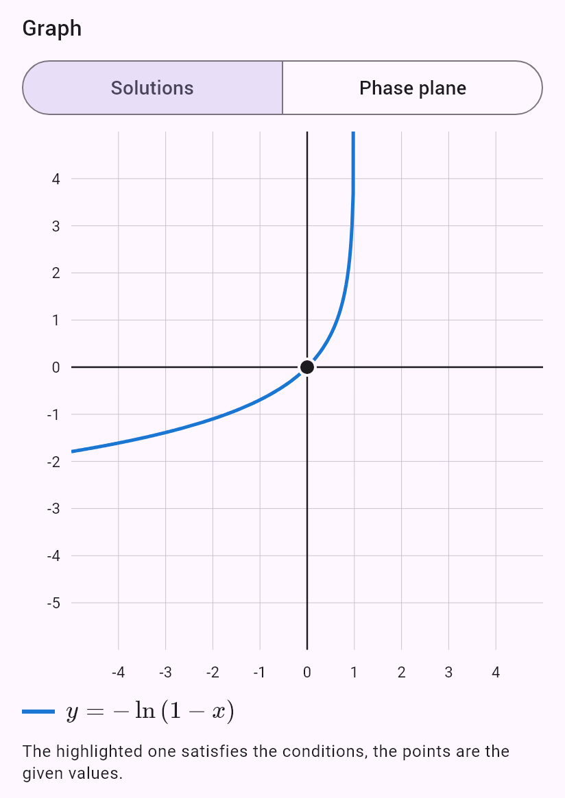
y'' = e^(2y), y(0) = 0, y'(0) = 1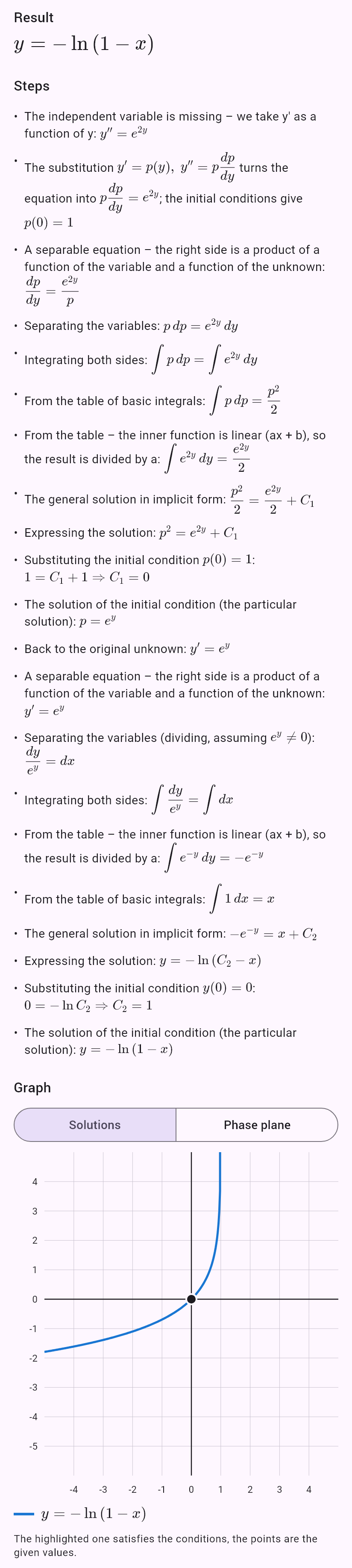
y'' + 2δy' + ω^2y = 0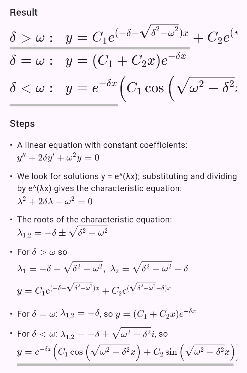
y'' + ω^2y = cos(2t)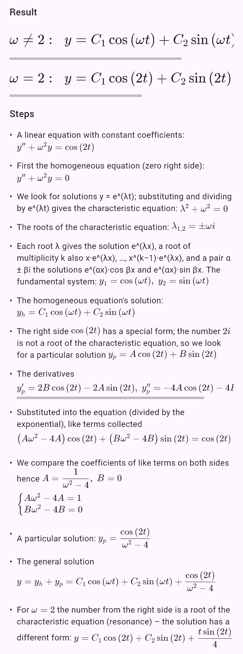
(1-x^2)y'' - 2xy' + 2y = 0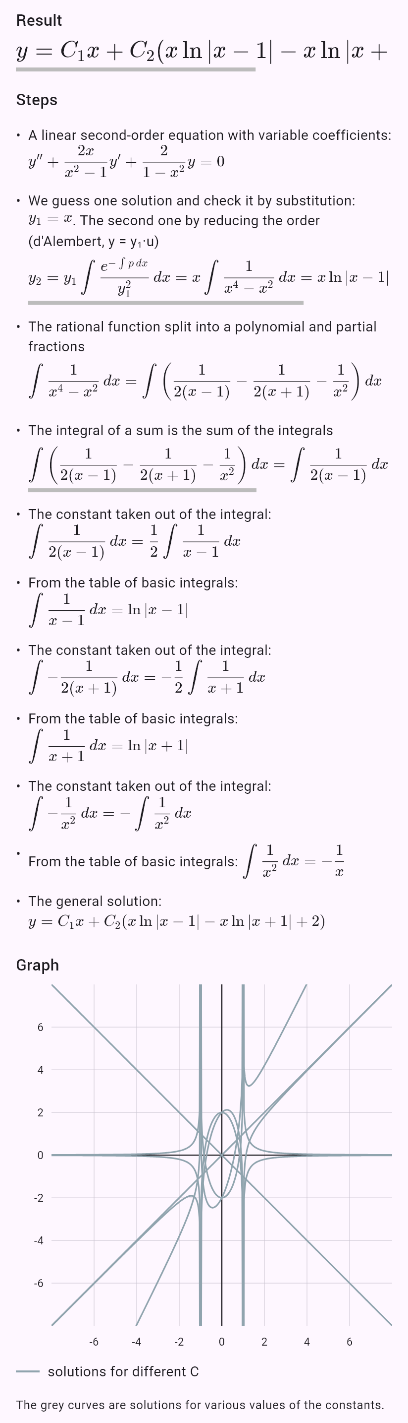
Known limitations
- An equation that needs a hint from the problem (other than z = ln y) can't be solved yet.
- For an equation with a parameter (k, λ, ω) the app draws no graph and takes the parameters as positive.
- Where the solution can't be expressed explicitly, it stays implicit.
- The Laplace transform doesn't know the Heaviside function, shifts and periodic right sides yet.